Image Processing and Recognition

C.J.C. Burges, "A tutorial on Support Vector Machines for pattern recognition", Kluvier (???) p. 1-43

The theory of SVM arises from the question "Under what conditions, and how fast, does the empirical mean converges uniformly to the true mean?".

Suppose to have n observation pairs, (x_i, y_i). Assume that these are drawn independently from the same probability distribution P, ie, they are "iid". Ther task is to find a machine that learns the association x->y. Such a machine is described by a generic function f(x, a), where a denotes the parameters of the machine that are to be determined during the training. For example, a might be the weights of a neural network.

In a binary pattern recognition problem y can have two values, +1 or -1, and the loss (1/2)|y-f(x,a)| can be either 0 or 1. The following bound holds on the risk, with probability 1-u,
R(a) ≤ R_emp(a) + [(h(1+log(2N/h))-log(u/4))/N]^1/2
where h is a non-negative integer, called the Vapnik-Chervonenkis dimension of the data. This results gives a method for choosing the machine that minimizes the right hand side bound on the risk (for a fixed sufficiently small u).

Remark. For a set of functions {f(a)} the VC dimension d_VC is defined as the maximum number of points that can be "shattered" by functions in the set, ie, such that for any binary class assignment of the points there is a function in the set which separates the points of the two classes. Note that this is not to say that any set of d_VC points can be shattered.

The VC dimension is an index of the capacity of the set of functions. For example the K nearest neighbor classifier (with K=1) has infinite VC dimension, and zero empirical risk. The K-nn classifier performs well.

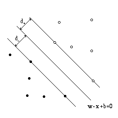Supose that the set of training points are linearly separable, ie, there exists a plane wx+b=0 such that the points x_i with y_i=1 ("positive" points) lay on one side and those with y_i=-1 ("negative" points) on the other side. w is the normal to the plane and |b|/|w| is the distance of the origin from the plane. Let d₊ and d_- be the shortest distances of the positive and negative points, respectively, from the separating plane. The margin of the separating plane is m=d₊+d_-.

The support vector algorithm is the search for the plane parameters (b and w) that maximizes the margin. The constraints

x_i w + b	≥	+1	for y_i=+1
x_i w + b	≤	-1	for y_i=-1

can be formulated in a unified form, y_i ( x_i w + b ) ≥ 1 The margin turns out to be 2/|w|. Therefore it is maximum when teh norm of w is minimum. This is a constrained minimum, which can be formulated using Lagrangian multipliers a_i. The Lagrangian
L_P = 1/2 |w|² - ∑ a_i y_i ( x_i w + b ) + ∑ a_i
must be minimized with respect to w, b, requiring dL_P/da_i = 0, and subject to the constraints a_i ≥ 0 (because the original constraints are inequalities).

It is convenient to cast the problem in the dual form, by solving the equations dL_P/dw=0 and dL_P/db=0. The dual Lagrangian
L_D = ∑ a_i - 1/2 ∑ a_i a_j y_i y_j x_i x_j
must be maximized with respect to a_i (in the subspace of positive a_i), subject to the constaint (that derives from dL_P/db=0) ∑ a_i y_i = 0 In the solution the point for which a_i>0 are the "support vectors" and lie on two planes (one "positive" one "negative") parallel to the separating plane. The others lie on the respective sides of these planes.

The solution to this problem is equivalent to the KKT (Karush-Kuhn-Tucker) conditions (because it satifyes a certain technical regularity condition),

dL_P/dw = w - ∑ a_i y_i x_i	=	0
dL_P/db = - ∑ a_i y_i	=	0
y_i ( x_i w + b ) - 1	≥	0
a_i	≥	0
a_i ( y_i ( x_i w + b ) - 1 )	=	0

The normal to the plane w is explicitly determined by the training set,
w = ∑ a_i y_i x_i
therefore it is the weigthed sum over the support vector points. The threshold b is determined by the last of the KKT conditions. In the test phase a point x is assigned to the "positive" or to the "negative" class depending on sgn(w x + b ).

If the training points are not separable, we cannot find a separating plane. We can relax the constraints allowing for some error, y_i ( x_i w + b ) ≥ 1 - e_i, and assign an extra cost for the errors, C(∑ e_i)^k, in the objective function L_P. This is a convex problem for any integer k. When k is 1 or 2 it is also a quadratic programming problem. If k=1, furthermore neither e_i, nor the associated multipliers appear in L_D.
L_P = 1/2 |w|² + C ∑ e_i - ∑ a_i ( y_i ( x_i w + b ) - 1 + e_i ) - ∑ u_i e_i
The KKT conditions are an extension of those for the separable case. In particular we have also

dL_P/de_i = C - a_i - u_i	=	0
e_i	≥	0
e_i u_i	=	0

Suppose that the training points are mapped in a (higher dimension) inner-product space,

A necessary and sufficient condition for the existance of H and F is the Mercer's condition: for any g with finite L₂ norm, ∫ K(x, y) g(x) g(y) dx dy ≥ 0 For example this condition is satisfied for positive integral powers of the dot product.